The purpose of these lessons is to learn more about multiple regression. We will work in the both the R and JASP statistical environments. For a text, we will rely on Andy Field's Discovering Statistics Using R and Barbara G. Tabachinik and Linda S. Fidell's Using Multivariate Statistics.
Note, you need to complete the Biomedical Statistics course before attempting this series of lessons.
Note, you need to complete the Biomedical Statistics course before attempting this series of lessons.
1. Correlation
Reading: Field, Chapters 6
Watch: Video on Correlation
In R, load the data HERE into a table called data.
Let's plot the data using the following command: plot(data)
You should see something that looks like the plot below.
Watch: Video on Correlation
In R, load the data HERE into a table called data.
Let's plot the data using the following command: plot(data)
You should see something that looks like the plot below.
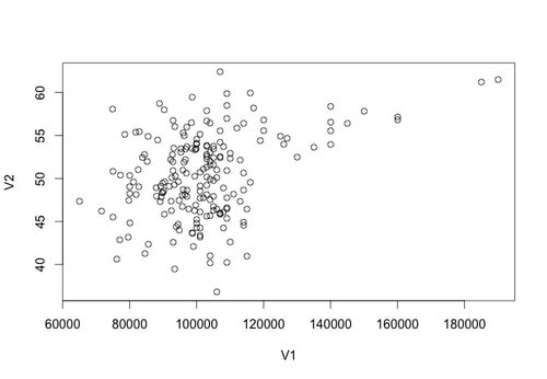
In statistics, sometimes we interested in the relationship between two variables. For example, is there a relationship between income and happiness? Is there a relationship between average hours of sleep per night and grade point average?
To test the extent of a relationship in statistics we use correlation. A Pearson correlation analysis return a number, "r", between -1 and 1 that represents the extent of a relationship. Positive numbers reflect a relationship wherein both the X and Y variables increase concomitantly. Negative numbers reflect a relationship wherein while one number variable increases the other decreases. A Pearson value of 0 suggests there is no relationship. However, the following relationship "strengths" are typically used:
0.1 to 0.3 = Weak correlation
0.3 to 0.5 = Medium correlation
0.5 to 1.0 = Strong correlation
The same ranges are true for negative correlations.
Returning a correlation value in r is very easy. Try: cor(data$V1,data$V2)
You will see that there is a medium strength correlation of 0.3585659 between these two variables.
In addition to interpreting correlations using the above ranges you can also use a formal statistical test against the null hypothesis. You do this by typing: cor.test(data$V1,data$V2)
You should see that the p value in this case is less than 0.001 indicating that the correlation of the sample differs from zero.
Correlation Assumptions
To perform a correlation analysis, there are two key assumptions: 1. the data must be interval or continuous and 2. the data for each variable must be normally distributed (there are a few exceptions but this is normally true). You can test the assumption of normality several ways.
Most people think that the assumption of normality means that you data is normally distributed, but it does not. What it actually means is that the sampling distribution of the mean for your data is normally distributed. Now recall, what we discussed before - the population data is normally distributed, then the sampling distribution of the mean will be normally distributed. So, if you know this "truth" then you actually do not need to test this assumption at all. But... do we actually know this, probably not. But what if the population data is skewed? Well, we also learned that if your sample size is greater than 30 (50 would be better), then the sampling distribution of the mean for the population will be normal even though the population data is not normally distributed.
So, what in practice do you do?
1. Use a sufficient sample size (n > 30, ideally 50: NOTE PER GROUP, NOT TOTAL). This is why in a lot of papers you do not even see a footnote saying that this assumption was tested.
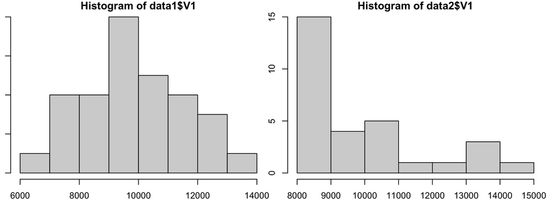
2. Plot a histogram of your data of your data. If the data looks normally distributed, then it most likely is. Assume the assumption is met. If it is not, and your sample size is less than 30... you can hope that point 1 is true.
Download the data files HERE and HERE.
Use the following R code:
data1<-read.table("normaldata.txt")
data2<-read.table("skewdata.txt")
par(mfrow=c(2, 2))
par(mar=c(1,1,1,1))
hist(data1$V1)
hist(data2$V1)
You clearly see from the plot that data1 is normally distributed and data2 is skewed quite badly. So, with data1 you would assume the assumption is met, with data2 - with a sample size of 30 - you would hope it is met. Your plot should look like the image below.
To test the extent of a relationship in statistics we use correlation. A Pearson correlation analysis return a number, "r", between -1 and 1 that represents the extent of a relationship. Positive numbers reflect a relationship wherein both the X and Y variables increase concomitantly. Negative numbers reflect a relationship wherein while one number variable increases the other decreases. A Pearson value of 0 suggests there is no relationship. However, the following relationship "strengths" are typically used:
0.1 to 0.3 = Weak correlation
0.3 to 0.5 = Medium correlation
0.5 to 1.0 = Strong correlation
The same ranges are true for negative correlations.
Returning a correlation value in r is very easy. Try: cor(data$V1,data$V2)
You will see that there is a medium strength correlation of 0.3585659 between these two variables.
In addition to interpreting correlations using the above ranges you can also use a formal statistical test against the null hypothesis. You do this by typing: cor.test(data$V1,data$V2)
You should see that the p value in this case is less than 0.001 indicating that the correlation of the sample differs from zero.
Correlation Assumptions
To perform a correlation analysis, there are two key assumptions: 1. the data must be interval or continuous and 2. the data for each variable must be normally distributed (there are a few exceptions but this is normally true). You can test the assumption of normality several ways.
Most people think that the assumption of normality means that you data is normally distributed, but it does not. What it actually means is that the sampling distribution of the mean for your data is normally distributed. Now recall, what we discussed before - the population data is normally distributed, then the sampling distribution of the mean will be normally distributed. So, if you know this "truth" then you actually do not need to test this assumption at all. But... do we actually know this, probably not. But what if the population data is skewed? Well, we also learned that if your sample size is greater than 30 (50 would be better), then the sampling distribution of the mean for the population will be normal even though the population data is not normally distributed.
So, what in practice do you do?
1. Use a sufficient sample size (n > 30, ideally 50: NOTE PER GROUP, NOT TOTAL). This is why in a lot of papers you do not even see a footnote saying that this assumption was tested.
2. Plot a histogram of your data of your data. If the data looks normally distributed, then it most likely is. Assume the assumption is met. If it is not, and your sample size is less than 30... you can hope that point 1 is true.
Download the data files HERE and HERE.
Use the following R code:
data1<-read.table("normaldata.txt")
data2<-read.table("skewdata.txt")
par(mfrow=c(2, 2))
par(mar=c(1,1,1,1))
hist(data1$V1)
hist(data2$V1)
You clearly see from the plot that data1 is normally distributed and data2 is skewed quite badly. So, with data1 you would assume the assumption is met, with data2 - with a sample size of 30 - you would hope it is met. Your plot should look like the image below.
3. Another graphical test you can do to test normality is a Q-Q plot. Try the following with the data you have loaded.
install.packages("car")
library(car)
par(mfrow=c(2, 2))
par(mar=c(1,1,1,1))
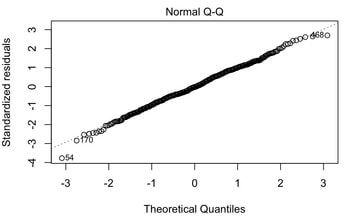
qqPlot(data1$V1)
qqPlot(data2$V1)
Interpreting a Q-Q plot is pretty straightforward. Ideally, if your data is all in a straight line, it is normally distributed. If it has a weird shape and is curved, and especially if it falls outside the confidence window, then your data is not normally distributed. You should see clearly in the Q-Q plot that data1 is normal and that data2 is not.
install.packages("car")
library(car)
par(mfrow=c(2, 2))
par(mar=c(1,1,1,1))
qqPlot(data1$V1)
qqPlot(data2$V1)
Interpreting a Q-Q plot is pretty straightforward. Ideally, if your data is all in a straight line, it is normally distributed. If it has a weird shape and is curved, and especially if it falls outside the confidence window, then your data is not normally distributed. You should see clearly in the Q-Q plot that data1 is normal and that data2 is not.
4. You can also statistically test your data for normality. One way to assess normality is to use a Shapiro Wilk test (see HERE). The Shapiro Wilk test assesses the normality of a data set and provides a p value - a test statistic that we will talk a lot more about later - that the states whether or not the data is normally distributed. If the p value of the test is less than 0.05 then the data is not normally distributed. If the p value of the test is greater than 0.05 then the data is normally distributed. Try a Shapiro Wilk test on your data by doing this: shapiro.test(data1$V1).
You should see the p-value is 0.9163 which means according to the Shapiro Wilk test data1 is normally distributed. Now try it for data2 shapiro.test(data2$V1). You should see that the p-value is significant (p-value = 8.788e-05) meaning that data is not normally distributed.
Another way to test normality is via a Kolmogorov-Smirnov test. The KS test compares your data against a distribution of your choice (e.g., normal). With this test, you must specify the mean and the standard deviation of the distribution so you need to use the values from your data to approximate those.
Try this with data1: ks.test(data1$V1,pnorm,mean(data1$V1),sd(data1$V1))
You should see that the test is not significant so again, data1 is normal according to the KS test. Note "pnorm" just means you are comparing to a normal distribution. The KS test can actually be used to test against any distribution, not just the normal one.
Now try it with data2: ks.test(data2$V1,pnorm,mean(data2$V1),sd(data2$V1))
You will see that this test is also not significant. But why? The KS test is better for large samples of data (n > 100) and it does not handle heavily skewed data very well. This is because the mean and the standard deviation you are using are biased by the skew.
But try this: ks.test(data2$V1,pnorm,median(data2$V1),sd(data2$V1))
You should see that the p value is now significant (p-value = 0.003172). The median is a better approximation of the centre of the distribution given the skew.
SOME FINAL NOTES. If you have multiple groups, do not forget you have to test the assumption for each group. Most statistical test are robust against violations of the assumption of normality. In other words, the tests will probably work if this test is failed.
For additional info on the assumption of normality:
WATCH THIS
READ THIS
Non Parametric Correlation Tests
So, what do you do if you fail the assumption of normality? You run a non-parametric correlation test. The two most common ones to use are Spearman's Correlation Coefficient and Kendall's Tau. In R:
cor(data$V1, data$V2, method = "spearman")
or
cor(data$V1, data$V2, method = "kendall")
Point Serial and Biserial Correlations
I am not going to write a lot here, but basically point serial and biserial correlations are used when one of the two variables you want to correlate is dichotomous. Point serial correlations are used when one variable is a discrete dichotomy and biserial correlations are used when one variable is a continuous dichotomy.
Assignment
1. The data HERE contains 6 columns of numbers. Test the correlation between column 1 and the other columns. Report both the relationships as defined above and also the p values for each correlation test.
Things to Understand
1. What is covariance?
2. What is meant by standardization?
3. What is a correlation coefficient?
4. Understand how a t-test for correlation works.
5. Understand how a confidence interval for a correlation coefficient is computed.
6. What is the causality problem?
7. What are the assumptions of correlation?
8. What are point serial and biserial correlations?
2. Partial Correlations
Reading: Field, Chapter 6
Watch: Partial Correlations
Partial correlations are used when you want to examine the relationship between two variables while controlling for a third. Another way to say this is, a correlation between two variables in which the effects of other variables are held constant is known as a partial correlation.
Read the data HERE into a table. This data contains column headers so use the following command:
data = read.table('examanxiety.txt',header = TRUE)
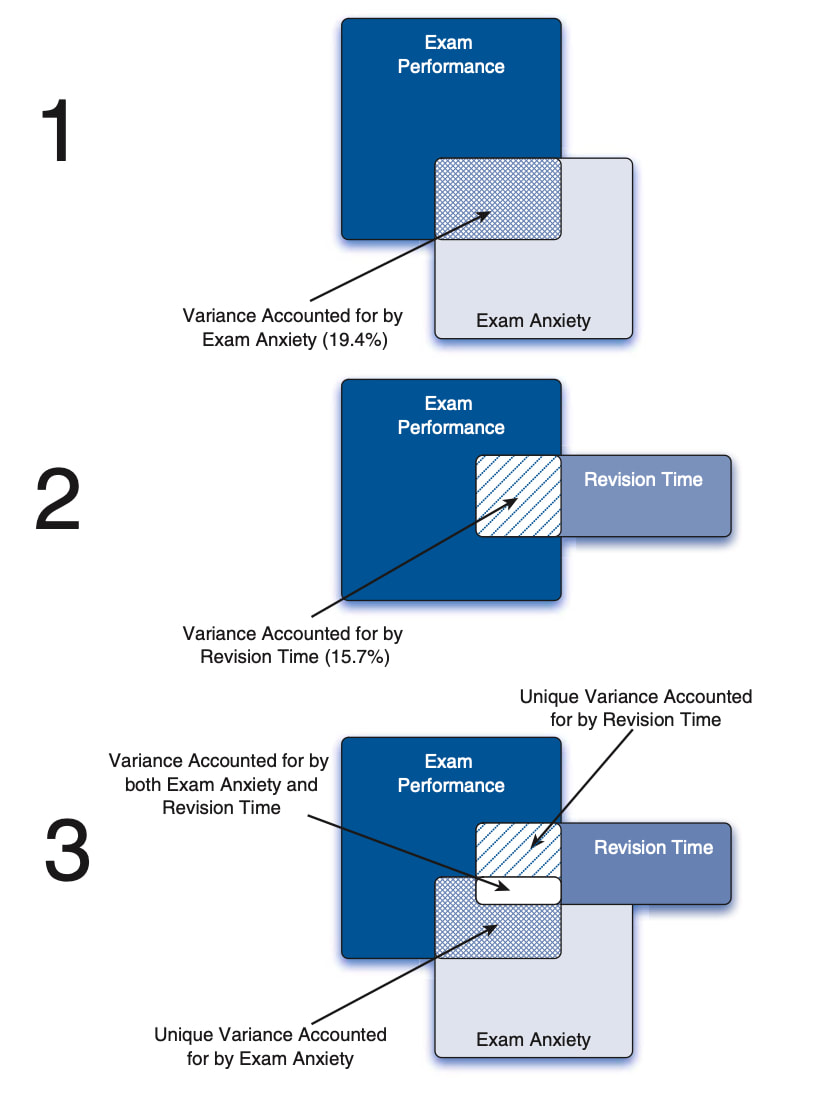
The data reflects contains fives columns - the three we are interested in for now are exam anxiety (data$Anxiety), exam revision time (data$Revise), and exam performance (data$Exam). There are correlations between anxiety and exam performance (-0.44) and revision time and exam performance (0.39). Check these now.
Before we go further we should talk about what r^2 means. r squared is known as the proportion of explained variance or the coefficient of determination. So, with the above data anxiety explains 19.4% of the variance in exam performance (0.44 * 0.44) and revision time explains 15.2% of the variance in exam performance.
But what is we wanted to know the impact of anxiety on exam performance while controlling for revision time? This is where partial correlations come in.
Watch: Partial Correlations
Partial correlations are used when you want to examine the relationship between two variables while controlling for a third. Another way to say this is, a correlation between two variables in which the effects of other variables are held constant is known as a partial correlation.
Read the data HERE into a table. This data contains column headers so use the following command:
data = read.table('examanxiety.txt',header = TRUE)
The data reflects contains fives columns - the three we are interested in for now are exam anxiety (data$Anxiety), exam revision time (data$Revise), and exam performance (data$Exam). There are correlations between anxiety and exam performance (-0.44) and revision time and exam performance (0.39). Check these now.
Before we go further we should talk about what r^2 means. r squared is known as the proportion of explained variance or the coefficient of determination. So, with the above data anxiety explains 19.4% of the variance in exam performance (0.44 * 0.44) and revision time explains 15.2% of the variance in exam performance.
But what is we wanted to know the impact of anxiety on exam performance while controlling for revision time? This is where partial correlations come in.
To actually run partial correlations in R you need to install a few things. Do the following:
install.packages("BiocManager")
BiocManager::install("graph")
install.packages("ggm")
library(ggm)
The function we need pcor is in the ggm package. We also need our data in a slightly different format, so execute the following commands:
examData = read.delim("examanxiety.txt", header = TRUE)
examData2 <- examData[, c("Exam", "Anxiety", "Revise")]
Now finally, you can see the partial correlation between exam scores and anxiety while controlling for revision time using the following:
pcor(c("Exam", "Anxiety", "Revise"), var(examData2))
You could square the output of this to get the proportion of explained variance for this relationship. You will also note that the output (-0.25) is considerably less than the correlation between anxiety and exam score (-0.44) because revision time clearly had an impact.
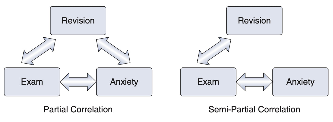
Note that partial correlations are not the same as semi-partial correlations which we will cover next but the diagram below might give you a hint as to the difference.
install.packages("BiocManager")
BiocManager::install("graph")
install.packages("ggm")
library(ggm)
The function we need pcor is in the ggm package. We also need our data in a slightly different format, so execute the following commands:
examData = read.delim("examanxiety.txt", header = TRUE)
examData2 <- examData[, c("Exam", "Anxiety", "Revise")]
Now finally, you can see the partial correlation between exam scores and anxiety while controlling for revision time using the following:
pcor(c("Exam", "Anxiety", "Revise"), var(examData2))
You could square the output of this to get the proportion of explained variance for this relationship. You will also note that the output (-0.25) is considerably less than the correlation between anxiety and exam score (-0.44) because revision time clearly had an impact.
Note that partial correlations are not the same as semi-partial correlations which we will cover next but the diagram below might give you a hint as to the difference.
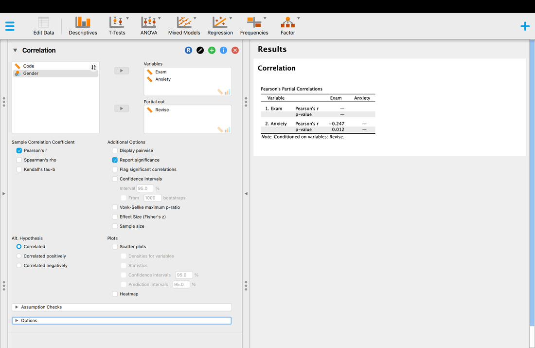
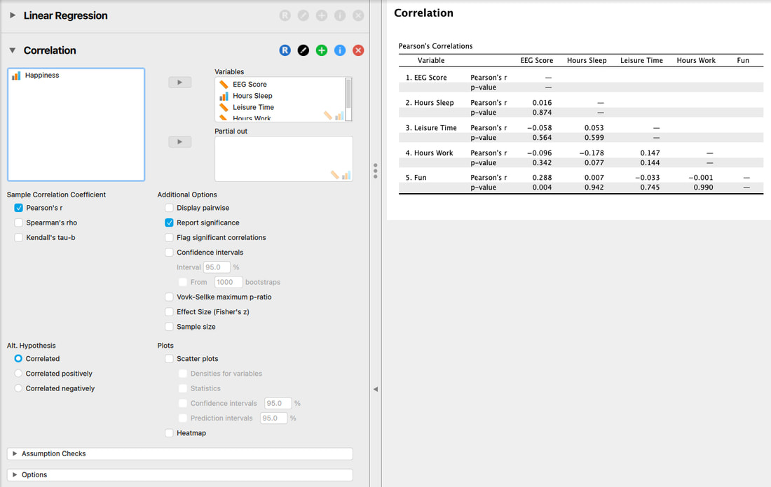
JASP
As you might image, this is considerably easier to do in JASP. I will leave it to you to figure out, but the image below should show you what to do to replicate what we have just done in R. You will note you can compute effect sizes, confidence intervals, or anything else you might need.
As you might image, this is considerably easier to do in JASP. I will leave it to you to figure out, but the image below should show you what to do to replicate what we have just done in R. You will note you can compute effect sizes, confidence intervals, or anything else you might need.
Assignment
1. Using the data from the first assignment, compute a partial correlation between the first two variables in the data set while controlling for the third.
2. Make sure you can do everything so far in JASP.
Things to Know
1. What is a partial correlation?
2. What is the coefficient of determination / proportion of explained variance?
3. Regression
READ: Field, Chapter 7
Watch THIS and THIS.
Slides are HERE.
Linear regression is closely related to correlation. Recall that in correlation we sought to evaluate the relationship between two variables - let's call then X and Y for simplicity. If a relationship is present then there is a Pearson r value less than -0.1 or greater than 0.1 - if no relationship is present then the Pearson r value falls between -0.1 and 0.1.
In regression, we seek to determine whether X can predict Y. For instance, do GRE scores predict success at graduate school? Do MCAT scores predict success at medical school? Does income predict happiness?
The general form of regression is Y = B0 + B1X. Hopefully you remember that this is essentially the equation of a line - the formula you learned in high school would have been Y = MX + B, which can be rewritten as Y = B + MX. In regression models, B0 is a constant and B1 is the coefficient for X. Think of it this way - income may range from $0 to $1,000,000 in our data and our happiness score might only range from 1 to 5. Thus, the regression model needs to tweak the income scores by multiplying them by B1 and adding B0 to predict a score between 1 and 5.
Another way to think of this is: output = model + error.
Load the data HERE into JASP. The data shows a column of scores called Calories and Attitude. We want to see if the Calories consumed on average PREDICTS Attitude.
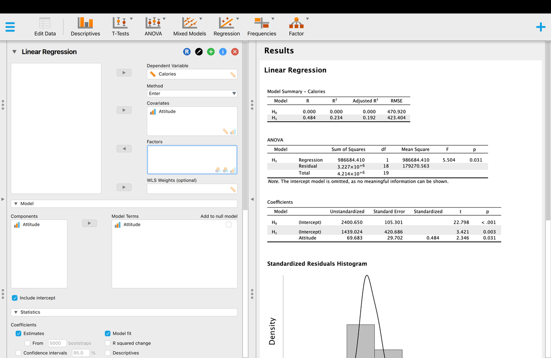
So what does all this mean? What JASP is doing is comparing a Null Model (Ho) which is simply the intercept on its own against a regression model where Calories is used to predict Attitude (H1). If you look at the ANOVA table it shows that there is a model that fits (p = 0.031). So, Calories do predict Attitude to some extent. It also shows that the model explains 23.4 % of the variance which is not that great. Note, that the adjusted R^2 value corrects for factors in the model of predictors and is a more accurate estimate in most instanced and is always lower - 19.2% in this case.
It also does a test on the coefficient but this test does not mean much as we only have one predictor variable, Calories. And, this is the same test statistic as F = T^2 (you can check this out). The technical name for this variable is that it is a regression coefficient.
Make sure you really understand correlation and regression BEFORE you tackle the assumptions of multiple regression.
4. Regression Assumptions Part One
Read: Field, Chapter 7
Also Read; Tabachnik and Fidell, Chapter 5
Use this DATA to test the assumptions below.
Regression and Multiple Regression come with a lot of assumptions, some which are easy to test and some which are not as easy to test (see Berry, 1993).
Assumption One: Variable Types
All predictor variables must be quantitative or categorical (with two categories), and the outcome variable must be quantitative, continuous and unbounded. By ‘quantitative’ I mean that they should be measured at the interval level and by ‘unbounded’ I mean that there should be no constraints on the variability of the outcome. If the outcome is a measure ranging from 1 to 10 yet the data collected vary between 3 and 7, then these data are constrained. If this assumption is broken for the types of variables, remove the variable. If the constrainment assumption is broken, consider removing the variable or proceed with caution.
You could check this easily by assessing the range of your predictor variables and ensuring this range is great than or equal to the range of the outcome variable. You can test this easily with the data set above using a "range" command in EXCEL, R, etc.
Assumption Two: Non-Zero Variance
The predictors should have some variation in value (i.e., they do not have variances of 0). Variables that break the assumption must be removed.
Again, you can test this easily with the data set above by using a command to calculate variance (var in R, etc).
Assumption Three: Multicolinearity
Essentially, the correlations between predictor variables should not be too high. For some, correlations more than 0.6 are considered bad. For others, correlations less than 0.8 are considered to be acceptable. There is no perfect answer here.
Note, perfect collinearity is when one predictor variable correlates perfectly with another predictor variable or combination of predictor variables.
One way to test multicollinearity is by looking at the correlation matrix data for the data. Try that with the data provided.
Another way to test multicollinearity is to look at the variance influence factor (VIF). Scores above 10 are considered to be very bad. With that said, any value above 1 should be investigated further. We will compute this when we run a full multiple regression. Some programs provide a tolerance statistic which is simply 1/VIF so values on 0.1 or less are considered to be bad.
It is crucial to know that violations of this assumption bias the model considerably and must be dealt with.
What to do if the assumption is violated?
1. Do nothing, report the statistics, and proceed.
2. Remove a redundant variable.
3. Transform of combine variables. Instead of having variable 1 and variable 2 separate, combine them in some fashion (e.g., new variable = variable 1 / variable 2.
4. Increase your sample size.
Assumption Four: Homoscedasticity
This is a bit different from Independent Samples T-Tests and ANOVA where the dependent variable is on the sample scale for everyone and you could just look at the variance of the dependent variable. In regression, homoscedasticity is when at each level of the predictor variable(s), the variance of the residual terms should be constant. This just means that the residuals at each level of the predictor(s) should have the same variance.
You cannot test this assumption without running the multiple regression so we will come back to it later.
If a variable breaks this assumptions, you would have to consider removing it from the model.
5. Regression Assumptions Part Two
Read: Field, Chapter 7
Also Read; Tabachnik and Fidell, Chapter 5
Use this DATA to test the assumptions below.
Regression and Multiple Regression come with a lot of assumptions, some which are easy to test and some which are not as easy to test (see Berry, 1993).
Assumption Five: Independence of Errors
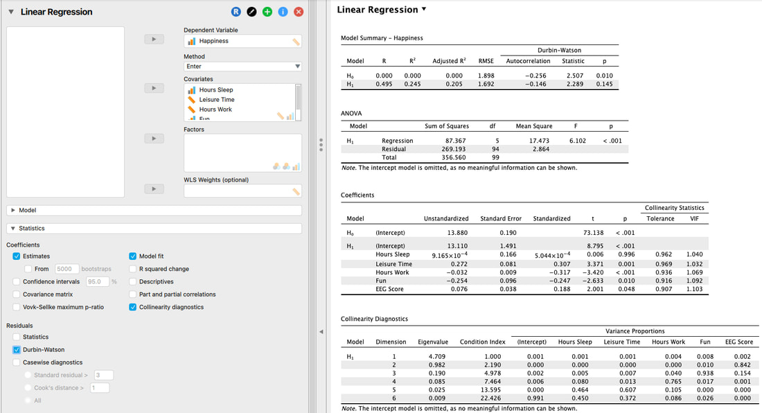
For any two observations the residual terms should be uncorreated (or independent). This eventuality is sometimes described as a lack of autocorrelation. This assumption can be tested with the Durbin–Watson test, which tests for serial correlations between errors. Specifically, it tests whether adjacent residuals are correlated. The test statistic can vary between 0 and 4, with a value of 2 meaning that the residuals are uncorrelated. A value greater than 2 indicates a negative correlation between adjacent residuals, whereas a value less than 2 indicates a positive correlation. The size of the Durbin–Watson statistic depends upon the number of predictors in the model and the number of observations. As a very conservative rule of thumb, values less than 1 or greater than 3 are definitely cause for concern. Be very careful with the Durbin–Watson test, though, as it depends on the order of the data: if you reorder your data, you’ll get a different value.
We will test this assumption when we run a full multiple regression in the next lesson.
Assumption Six: Normally Distributed Errors
It is assumed that the residuals in the model are random, normally distributed variables with a mean of 0. This assumption simply means that the differences between the model and the observed data are most frequently zero or very close to zero, and that differences much greater than zero happen only occasion- ally. Some people confuse this assumption with the idea that predictors have to be normally distributed. Predictors do not need to be normally distributed.
A simple way to test this is with a histogram of the residuals. We will do this in the next lesson when we run a full multiple regression.
Assumption Seven: Independence
It is assumed that all of the values of the outcome variable are independent (in other words, each value of the outcome variable comes from a separate entity / person).
There is no real way to test this assumption, it is simply something you need to know to be true.
Assumption Eight: Linearity
The mean values of the outcome variable for each increment of the predictor(s) lie along a straight line. In plain English this means that it is assumed that the relationship we are modelling is a linear one. If we model a non-linear relation- ship using a linear model then this obviously limits the generalizability of the findings.
Again, you have to run the multiple regression to assess this which we will do next.
Also Read; Tabachnik and Fidell, Chapter 5
Use this DATA to test the assumptions below.
Regression and Multiple Regression come with a lot of assumptions, some which are easy to test and some which are not as easy to test (see Berry, 1993).
Assumption Five: Independence of Errors
For any two observations the residual terms should be uncorreated (or independent). This eventuality is sometimes described as a lack of autocorrelation. This assumption can be tested with the Durbin–Watson test, which tests for serial correlations between errors. Specifically, it tests whether adjacent residuals are correlated. The test statistic can vary between 0 and 4, with a value of 2 meaning that the residuals are uncorrelated. A value greater than 2 indicates a negative correlation between adjacent residuals, whereas a value less than 2 indicates a positive correlation. The size of the Durbin–Watson statistic depends upon the number of predictors in the model and the number of observations. As a very conservative rule of thumb, values less than 1 or greater than 3 are definitely cause for concern. Be very careful with the Durbin–Watson test, though, as it depends on the order of the data: if you reorder your data, you’ll get a different value.
We will test this assumption when we run a full multiple regression in the next lesson.
Assumption Six: Normally Distributed Errors
It is assumed that the residuals in the model are random, normally distributed variables with a mean of 0. This assumption simply means that the differences between the model and the observed data are most frequently zero or very close to zero, and that differences much greater than zero happen only occasion- ally. Some people confuse this assumption with the idea that predictors have to be normally distributed. Predictors do not need to be normally distributed.
A simple way to test this is with a histogram of the residuals. We will do this in the next lesson when we run a full multiple regression.
Assumption Seven: Independence
It is assumed that all of the values of the outcome variable are independent (in other words, each value of the outcome variable comes from a separate entity / person).
There is no real way to test this assumption, it is simply something you need to know to be true.
Assumption Eight: Linearity
The mean values of the outcome variable for each increment of the predictor(s) lie along a straight line. In plain English this means that it is assumed that the relationship we are modelling is a linear one. If we model a non-linear relation- ship using a linear model then this obviously limits the generalizability of the findings.
Again, you have to run the multiple regression to assess this which we will do next.
6. Multiple Regression
Read: Field, Chapter 7
Also Read; Tabachnik and Fidell, Chapter 5
With multiple regression you have an outcome variable as you did with simple regression. With multiple regression however, you have multiple predictor variables. The reason for doing this, is that you believe some or all of the predictor variables are a better predictor of the outcome variable than any individual variable. A multiple regression tests whether or not this is a true statement. In other words, a significant multiple regression suggests that there is a linear model wherein the predictor variables predict the outcome variable to some extent. A non-significant multiple regression suggests that there is no linear combination of predictor variables that predicts the outcome variable.
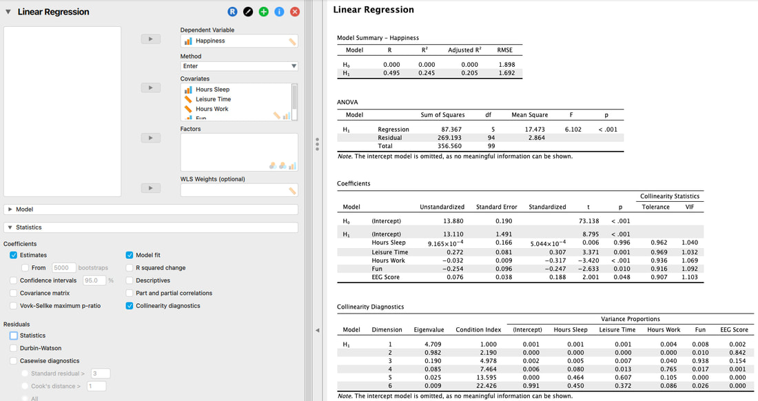
Load the data set HERE into JASP. You are running a study where you are trying to predict GRE scores from a variety of other measures. Can you do it? Running a multiple regression in JASP is also easy. Take a look at the image below.
Also Read; Tabachnik and Fidell, Chapter 5
With multiple regression you have an outcome variable as you did with simple regression. With multiple regression however, you have multiple predictor variables. The reason for doing this, is that you believe some or all of the predictor variables are a better predictor of the outcome variable than any individual variable. A multiple regression tests whether or not this is a true statement. In other words, a significant multiple regression suggests that there is a linear model wherein the predictor variables predict the outcome variable to some extent. A non-significant multiple regression suggests that there is no linear combination of predictor variables that predicts the outcome variable.
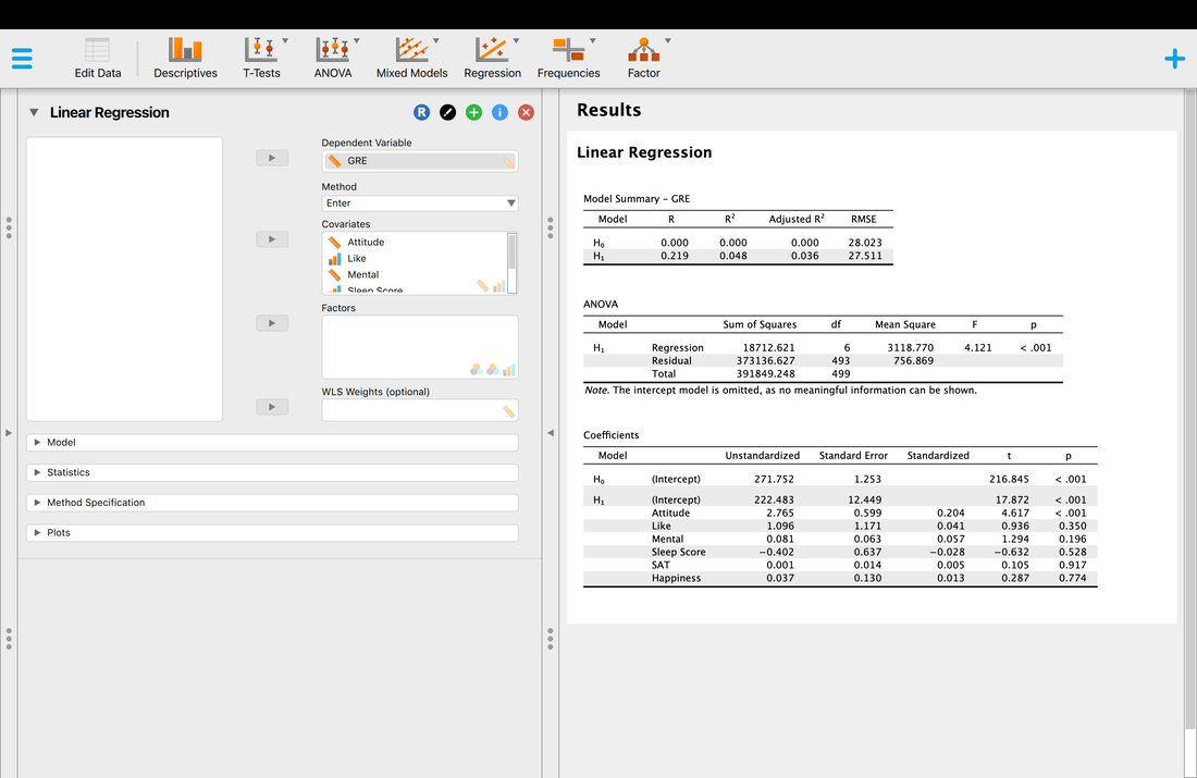
Load the data set HERE into JASP. You are running a study where you are trying to predict GRE scores from a variety of other measures. Can you do it? Running a multiple regression in JASP is also easy. Take a look at the image below.
So, lets walk through the output.
The model summary shows the comparison between H0, the null hypothesis model - that there is no linear combination of variables that predicts the outcome variable and H1, the alternative hypothesis that there is a linear combination of predictor variables that predicts the outcome variables. The model summary also shows the R and R^2 values for the alternative hypothesis, in this case 0.219 and 0.048, respectively. So, the model explains 4.8% of the variance in the outcome variable which is not great. If you use the conservative estimate of adjusted R^2, 0.036 or 3.6% of the variance you will see this is not a great model. Why do you think the values for H0 are all zero?
The ANOVA table is essentially a test as to whether the model for H1 explains significantly more variance than H0. In other words, that there is a model that fits the data. Here, we see that the regression model is significant, F = 4.121, p < 0.001. So, there is a model. And, you might get excited because p < 0.001. BUT, you have to remember that the model explained 4.8% of the variance which is VERY low.
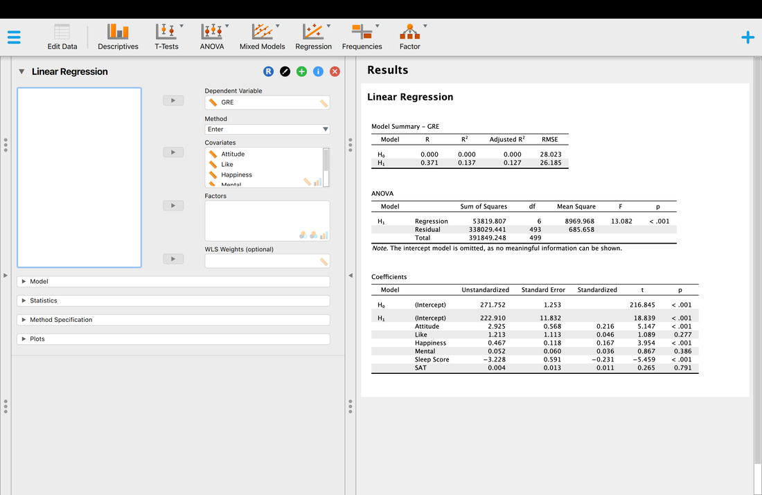
Finally, you might wonder which predictor variables really mattered. A simple assessment of this is to look at the test of the coefficients table. Basically, this is the individual relationship between each predictor variable and the outcome variable. For example, you will see that the p value for attitude is the only significant test, p < 0.001. All of the other variables are non-significant. So, you might be tempted to conclude that attitude is the only predictor of GRE scores. Is this a true statement. Let's look at a simple regression model where attitude predicts GRE scores.
The model summary shows the comparison between H0, the null hypothesis model - that there is no linear combination of variables that predicts the outcome variable and H1, the alternative hypothesis that there is a linear combination of predictor variables that predicts the outcome variables. The model summary also shows the R and R^2 values for the alternative hypothesis, in this case 0.219 and 0.048, respectively. So, the model explains 4.8% of the variance in the outcome variable which is not great. If you use the conservative estimate of adjusted R^2, 0.036 or 3.6% of the variance you will see this is not a great model. Why do you think the values for H0 are all zero?
The ANOVA table is essentially a test as to whether the model for H1 explains significantly more variance than H0. In other words, that there is a model that fits the data. Here, we see that the regression model is significant, F = 4.121, p < 0.001. So, there is a model. And, you might get excited because p < 0.001. BUT, you have to remember that the model explained 4.8% of the variance which is VERY low.
Finally, you might wonder which predictor variables really mattered. A simple assessment of this is to look at the test of the coefficients table. Basically, this is the individual relationship between each predictor variable and the outcome variable. For example, you will see that the p value for attitude is the only significant test, p < 0.001. All of the other variables are non-significant. So, you might be tempted to conclude that attitude is the only predictor of GRE scores. Is this a true statement. Let's look at a simple regression model where attitude predicts GRE scores.
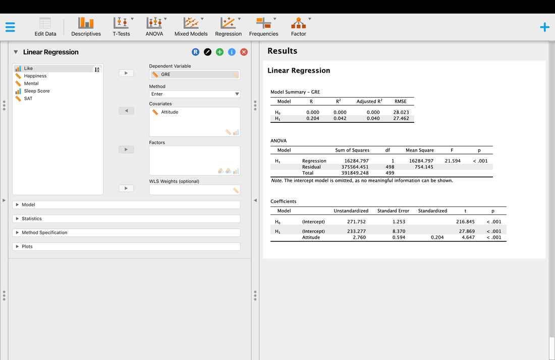
You will notice that the R and R^2 values are lower, and the individual statistics are close but slightly different.
So, just because attitude was the only significant predictor in the multiple regression, the other variables do contribute as well because a multiple regression is a linear combination of variables. This is where the unstandardized and standardized coefficients come in. The actual equation for a multiple regression is:
Y = B0 + B1X1 + B2X2 + B3X3 + B4X4 + B5X5 + B6X6 (I will include six predictors because that is what we have here.
The Beta values B0, B1, etc are the weights that each predictor variable is multiplied by when computing the predicted values of the outcome variable. First, think back to simple regression,
y = mx + b or in regression form Y = B0 + B1X1 where B0 is the constant, B1 is the "slope" and X1 is the x value. You multiply all this together to get y or the predicted y value.
So, in a multiple regression you use the formula in bold above for every row of data to compute the predicted outcome value.
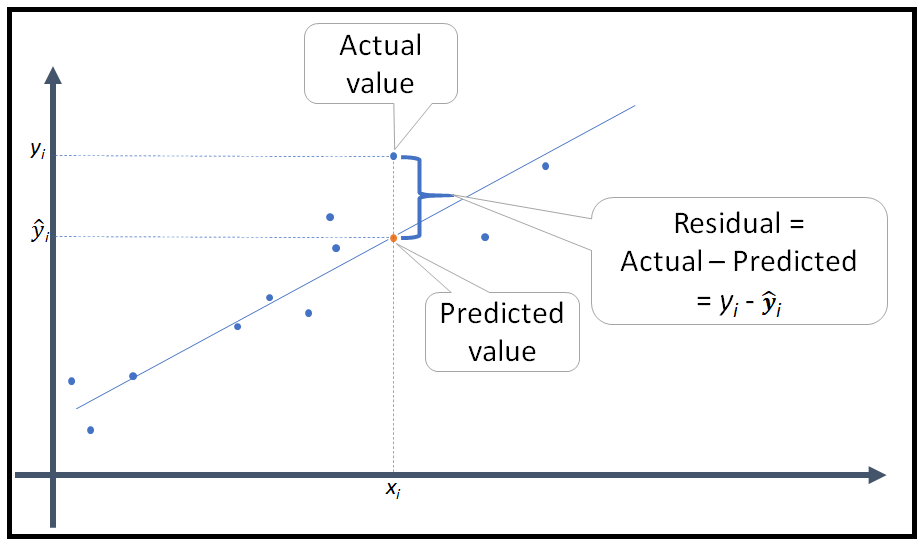
This is what residuals are, right? Ypredicted - Yactual = Error (residual). If you have a perfect multiple regression, R = 1, then Ypredicted - Yactual = 0. Make sure you understand this concept.
And, when a multiple regression is computed, the math underlying it is trying to minimize the error, or the residuals as this is the "best" fit of the model to the data.
So, the point I was trying to make is that while attitude is the only significant predictor, ALL of the predictor variables have some contribution to the multiple regression.
A final thought, the B coefficients have to be standardized because the predictor variables are all on different scales (usually).
Now, let's run a multiple regression on another DATA set, again, we are trying to predict GRE scores from the provided predictor variables.
So, just because attitude was the only significant predictor in the multiple regression, the other variables do contribute as well because a multiple regression is a linear combination of variables. This is where the unstandardized and standardized coefficients come in. The actual equation for a multiple regression is:
Y = B0 + B1X1 + B2X2 + B3X3 + B4X4 + B5X5 + B6X6 (I will include six predictors because that is what we have here.
The Beta values B0, B1, etc are the weights that each predictor variable is multiplied by when computing the predicted values of the outcome variable. First, think back to simple regression,
y = mx + b or in regression form Y = B0 + B1X1 where B0 is the constant, B1 is the "slope" and X1 is the x value. You multiply all this together to get y or the predicted y value.
So, in a multiple regression you use the formula in bold above for every row of data to compute the predicted outcome value.
This is what residuals are, right? Ypredicted - Yactual = Error (residual). If you have a perfect multiple regression, R = 1, then Ypredicted - Yactual = 0. Make sure you understand this concept.
And, when a multiple regression is computed, the math underlying it is trying to minimize the error, or the residuals as this is the "best" fit of the model to the data.
So, the point I was trying to make is that while attitude is the only significant predictor, ALL of the predictor variables have some contribution to the multiple regression.
A final thought, the B coefficients have to be standardized because the predictor variables are all on different scales (usually).
Now, let's run a multiple regression on another DATA set, again, we are trying to predict GRE scores from the provided predictor variables.

So, now we have a significant multiple regression where it looks like three of the predictor variables contribute to the model. But what if we want to know which variable matters the most? Examining the coefficient table and the t and p values is simply not good enough. In the next lesson, we will look at the way to address this - stepwise regression.
7. Stepwise Multiple Regression
Read: Field, Chapter 7
Also Read; Tabachnik and Fidell, Chapter 5
You might have noticed when you ran your last multiple regression that there was a box that specified the method as "Enter".
Also Read; Tabachnik and Fidell, Chapter 5
You might have noticed when you ran your last multiple regression that there was a box that specified the method as "Enter".
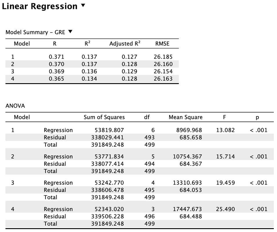
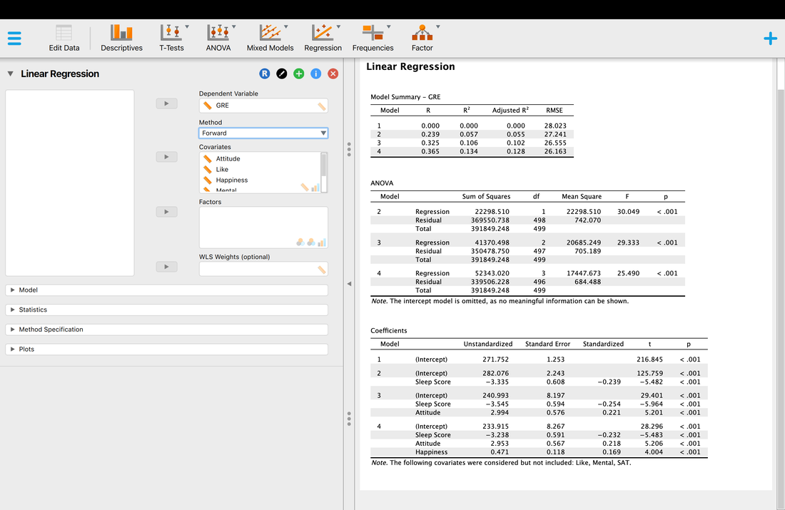
If you click on the down arrow beside "Enter" you will see that you can change the method to Backward, Forward, or Stepwise. Try selecting Backward.
|
|
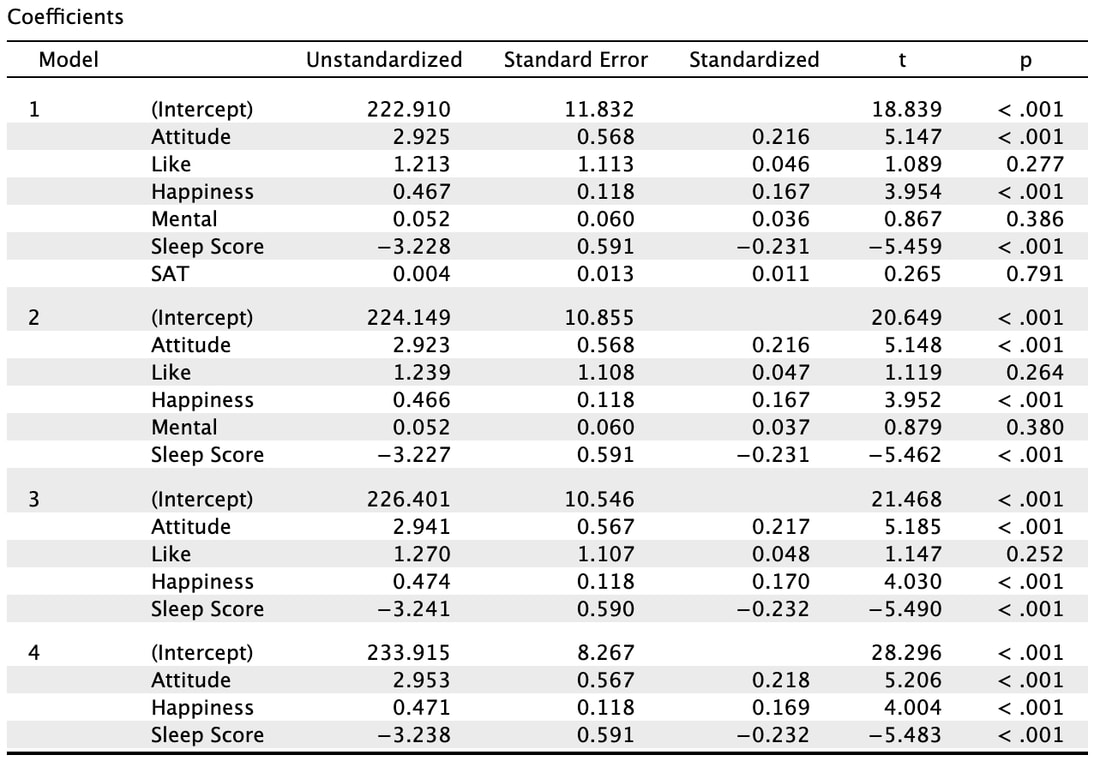
What the Backward method does is start with all the predictor variables in the model. That is model 1. You will note that all the statistics are the same as the Enter method. For model 2, the backward method removes a variable that does the least to help the accuracy of the multiple regressions prediction. In this instance, SAT was removed. You will note the R value has dropped slightly but the F statistic has increased indicating a better model fit. This process is repeated until removing a variable causes a significant change in the R and R^2 value. In other words, there would be a significant difference between model 4 and model 5 (which we do not see here, but you could do this manually in R). There is no significant difference between model 3 and model 4. So, the results of the backward regression tell us that we only need Attitude, Happiness, and Sleep Score to predict GRE results accurately. However, the backward regression does not tell us which of these variables is more important.
Let's rerun the regression using the Forward method.
Let's rerun the regression using the Forward method.
The Forward methods adds variables to the model until there is no significant difference in the R and R^2 values. So, in this case model 2 is significantly better than model 1. However, model 5 (which we do not see) is not significantly better than model 4. You will note that the same three variables comprise a model that best predicts GRE scores. Note however, while in this instance the models converged, this is not always the case because of how the variables interact. But, here you could argue that Sleep Score is the best predictor (or contributes the most) to the multiple regression.
Finally, let's try the Stepwise method.
Finally, let's try the Stepwise method.
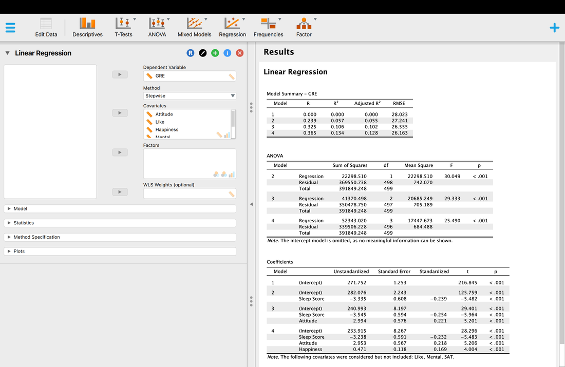
The results of the Stepwise method may appear similar (they are identical here) but there are underlying methodological differences between the Forward and Stepwise methods. Essentially, the Stepwise method iteratively tries all possible combinations of variables as opposed to simply adding one variable at a time. As a result, while it does here, the Forward and Stepwise methods so not always yield the same regression model. Read Tabachinik and Fidell Chapter 5 for more detail on the underlying math behind the Stepwise method.
8. Revisiting the Assumptions of Multiple Regression
Read: Field, Chapter 7
Also Read; Tabachnik and Fidell, Chapter 5
Use this DATA to test the assumptions below. With this data we are trying to predict happiness from a bunch of other measures.
Okay, now that we have run the multiple regression and understand it better, lets test all the assumptions we discussed previously.
However, before we begin testing all of the individual assumptions, lets cover what most people do to test the assumptions. A simple test of the assumptions is to examine the distribution of the residuals (the errors) in the models predictions.
The basic idea is that if the residuals are normally distributed, then one has met the assumptions of multiple regression. Doing this in JASP is easy. Note, it is better to look at the standardized residuals.
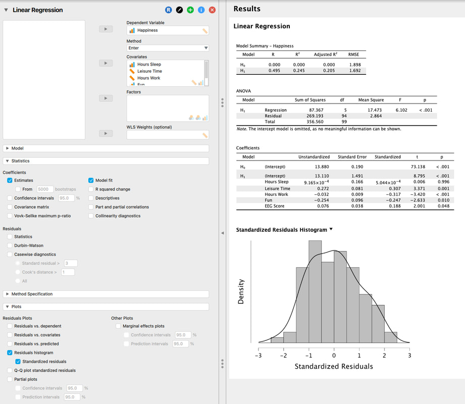
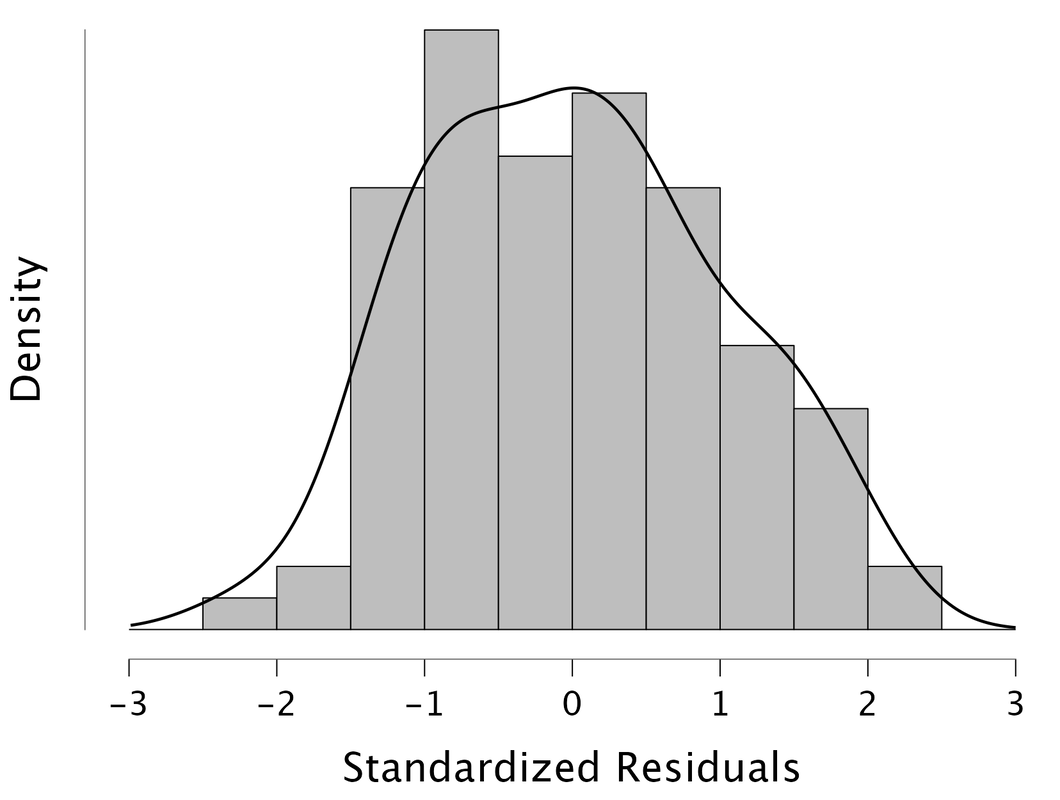
Here, we see that the residuals are normally distributed so we would "assume" that the assumptions of multiple regression are met. One could also look at a Q-Q plot of the standardized residuals.
The QQ plot, or quantile-quantile plot, is a graphical tool to help us assess if a set of data plausibly came from some theoretical distribution such as a normal or exponential. For example, if we run a statistical analysis that assumes our residuals are normally distributed, we can use a normal QQ plot to check that assumption. It's just a visual check, not an air-tight proof, so it is somewhat subjective. But it allows us to see at-a-glance if our assumption is plausible, and if not, how the assumption is violated and what data points contribute to the violation. Technically, a QQ plot is a scatterplot created by plotting two sets of quantiles against one another. If both sets of quantiles came from the same distribution, we should see the points forming a line that's roughly straight.
The QQ plot, or quantile-quantile plot, is a graphical tool to help us assess if a set of data plausibly came from some theoretical distribution such as a normal or exponential. For example, if we run a statistical analysis that assumes our residuals are normally distributed, we can use a normal QQ plot to check that assumption. It's just a visual check, not an air-tight proof, so it is somewhat subjective. But it allows us to see at-a-glance if our assumption is plausible, and if not, how the assumption is violated and what data points contribute to the violation. Technically, a QQ plot is a scatterplot created by plotting two sets of quantiles against one another. If both sets of quantiles came from the same distribution, we should see the points forming a line that's roughly straight.
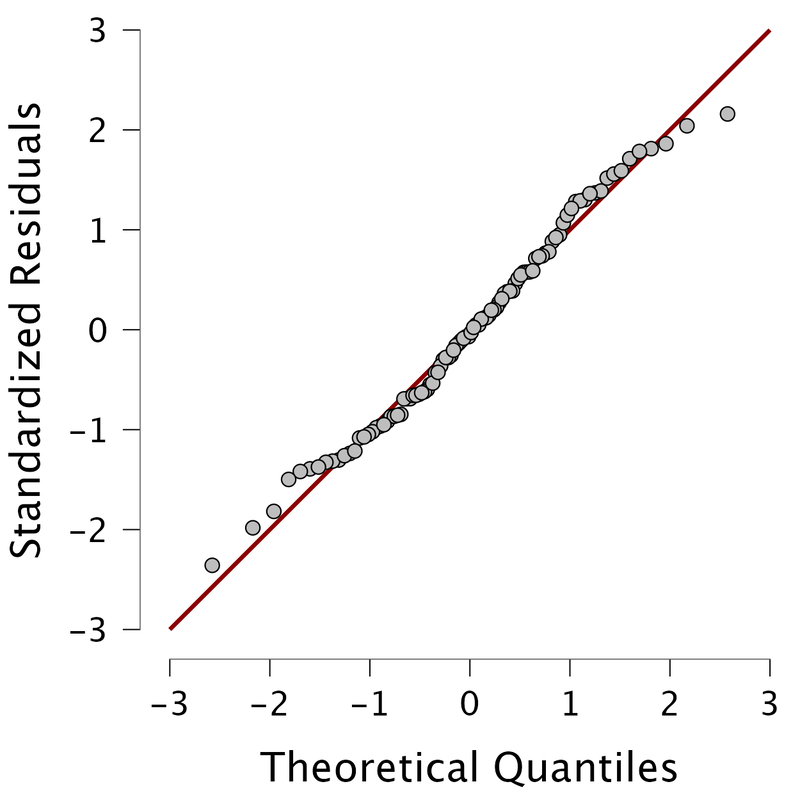
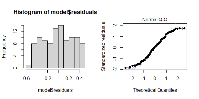
Because most of the points fall on the line, we would assume the residuals are normally distributed. Below, you see an example of where the residuals are not normally distributed. Note, these are graphic tests and as such, one has to take them for what they are.
Testing the Specific Assumptions
While the above methods are "easy", there are times where you need (or may be asked) to do more to test the individual assumptions.
1. Examine Influential Cases
Regression models are extremely biased by influential cases (i.e., outliers). To check for influential cases one can examine the individual standardized residuals or check the Cook's Distance for each data point.
When examining the individual standardized residuals you are essentially looking for a value greater than +3 or less than -3. Basically, if the error is too big, you assume there is an outlying variable that needs to be removed.
A Cook's Distance of greater than 1 is assumed to be bad. But what is a Cook's Distance? Technically, Cook’s Distance is calculated by removing the a data point from the model and recalculating the regression. It summarizes how much all the values in the regression model change when the an observation is removed.
In JASP, it is easy to examine the individual standardized residuals and Cook's distance.
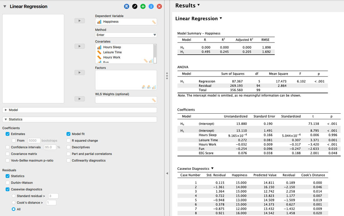
JASP even makes it easier - if you uncheck "All" it will only show you cases where the residuals or Cook's Distance violate your acceptable values (which you can change).
2. Multicolinearity
Checking for multicolinearity is very important, especially if you have a large number of predictor variables. There are two simple ways to check for multicolinearity. One, is to examine the correlation matrix and ensure there are no correlations between the predictor variables above 0.6 (conservative) or 0.8 (liberal). Note that the 0.6 and 0.8 values are rules of thumb and based on opinion.
There are no values above 0.6 here, let alone 0.8 so you can assume the assumption is not broken.
Another way to examine multicolinearity is to examine the colinearity diagnostics.
Another way to examine multicolinearity is to examine the colinearity diagnostics.
Explanation of this table is beyond the scope of this website, but it is covered in both texts. The short version is, you are looking for is a Condition Index greater than 15. There is one here. BUT, you also have to look at the variance proportions. If none are above 0.8 (some say 0.9) then you can assume you have met the assumption. In this case, you have as all of the variance proportions for Dimension 6 are below 0.8.
3. Independence of Errors
The assumption itself is outlined in a previous section, but this assumption can be tested with the Durbin Watson Test.
3. Independence of Errors
The assumption itself is outlined in a previous section, but this assumption can be tested with the Durbin Watson Test.
Here, we are simply looking at the Statistic and the p value. Ignore the output for H0, it is meaningless. But, we must examine H1. If the Statistic is between 1 and 3 and the p value is not significant, then the assumption is met.
The Other Assumptions
The other assumptions can be tested as outlined in previous sections or are simply assumed to be met if all of the tests here are met.
Assumption Failed?
If you fail an assumption, you need to do something about it. This might mean removing data in the case of influential cases or removing a variable in the case of multicolinearity.
9. Binary Logistic Regression
Read Field, Chapter 8.
Also read Tabachnik and Fidell, Chapter 10
The simplest way to explain binary logistic regression is this way - with traditional regression models we are predicting a continuous variable, in logistic regression we are predicting a categorical variable - whether someone is male or female for instance. In binary logistic regression we are predicting a categorical variable with only two levels, with multinomial logistic regression we would be predicting a categorical variable with three or more levels. Here, we will only be covering binary logistic regression.
Let's just dive in and run one. Download THIS data and open it in JASP.
This data set actually lists all 1313 passengers on the Titantic. It also lists the class they were in (1st, 2nd, etc), their age, and their sex. It also lists whether they survived or not. We are going to use binary logistic regression to see if we can predict survival based on the class they were in, their age, and their sex.
One thing to note, in logistic regression covariates reflect continuous variables (age in this instance) and factors reflect categorial variables (class, sex).
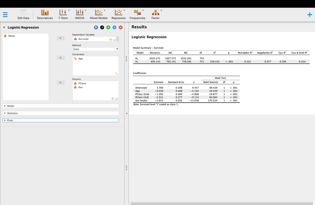
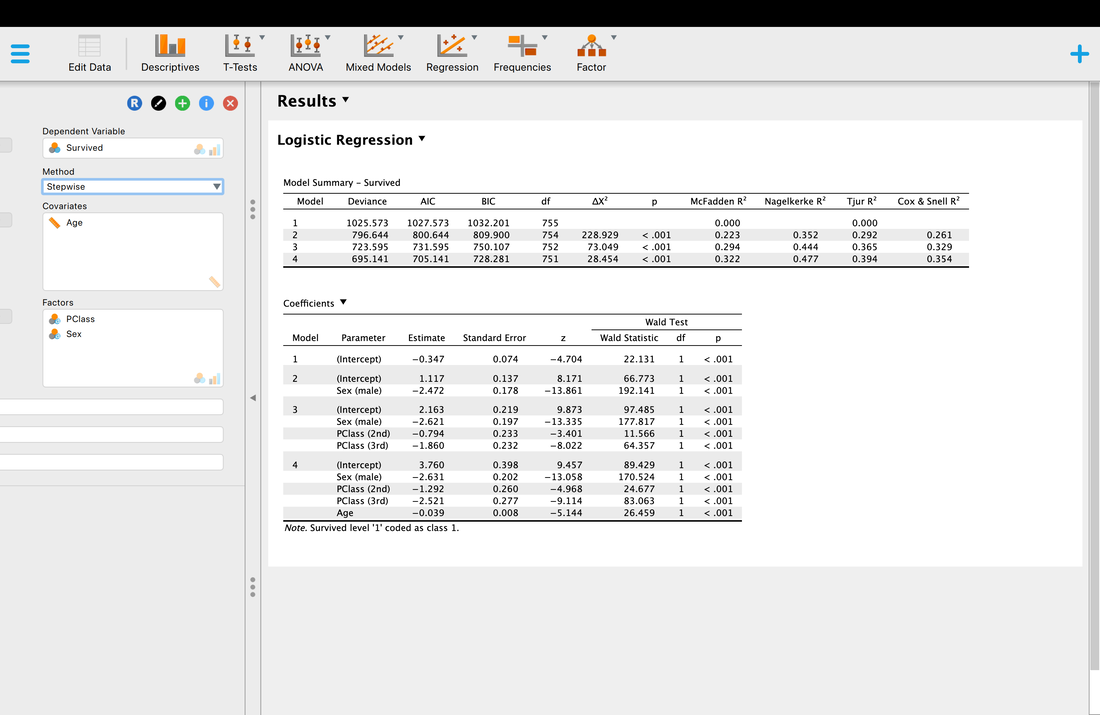
Well, the short version is p < 0.05 so there is a model that works, and yes, you can predict passenger survival from class, sex, and age.
You will notice that are a wide range of R2 values to choose from - McFadden, Nagelkerke, Tjur, Cox and Snell. You should know by now that R2 reflects the proportion of explained variance, but why is JASP reporting four different R2 values? Well, because people have argued about the correct way to compute R2 for logistic regression. Nagelkerke for instance is a correction to Cox and Snell. Sadly, there is no correct answer so the best guidance I can provide is to search the literature for a paper similar to the analysis you want to use and report the same measure they did and cite them.
But what of the other statistics? The Chi Squared statistic is just the test statistic for the model which we have discussed previously. However, it is based on log-likelihoods. The short version is, logistic regression works on the basis on comparing the observed versus predicted values - the observation of survival here versus the prediction of survival. The log-likelihood here is based on summing the probabilities associated with the predicted and actual outcomes (Tabachnick & Fidell, 2007). You can learn more about log-likelihoods HERE and HERE.
But AIC and BIC are new. AIC is Akaike Information Criteria, yet another statistic. But what does it measure? The problem with R2 is that the more predictor variables you add, significant or not, R2 will almost always go up. AIC is a measure of goodness of fit that penalizes a model the more predictor variables that are added. So, a model with fewer predictor variables might have a lower R2 value but also a lower AIC score which is good - lower AIC scores mean better model fit. The problem with AIC is that there is no scale for it for comparison, it is computed from the model itself. So, AIC is useful for comparing models that predict the same thing but useless for comparing models that predict different things. BIC is essentially a Bayesian (Bayesian Information Criteria) version of AIC.
Finally, as with multiple regression there is a test for each coefficient. These tests are reported with a Wald statistic. It is basically the test of the individual variables. If you want to learn more about why it is called a Wald statistic read Field!
As with multiple regression you can you stepwise regression - backward, forward, or stepwise to try and ascertain which variables contribute the most to the model - but in this instance as you can see below, they all do.
As with all statistical tests, logistic regression comes with assumptions which must be met.
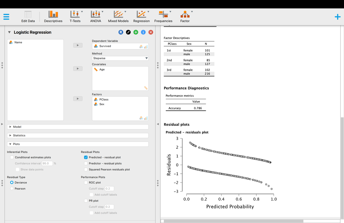
Assumption One. Linearity. In the case of logistic regression this is interesting because the outcome variable is categorical. As such, the assumption here is that there is a linear relationship between continuous predictor variables and the log (or logit) of the outcome variable. The easiest way to test this assumption is to look at the plot of the residuals and see that both lines are roughly linear (there are two lines because there are two outcomes).
Assumption One. Linearity. In the case of logistic regression this is interesting because the outcome variable is categorical. As such, the assumption here is that there is a linear relationship between continuous predictor variables and the log (or logit) of the outcome variable. The easiest way to test this assumption is to look at the plot of the residuals and see that both lines are roughly linear (there are two lines because there are two outcomes).
Assumption Two. Independence of Errors. This assumption is the same as for regression - each case has to be independent and unique.
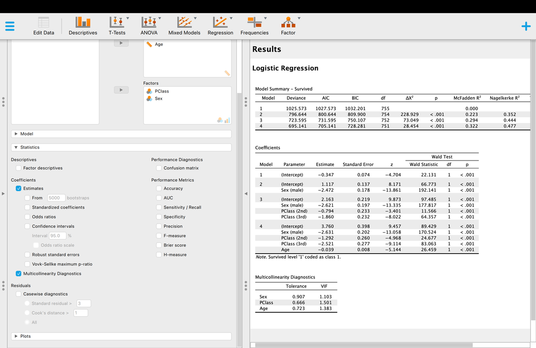
Assumption Three. Multicollinearity. Again, the same as with regression and this can be tested within JASP using the multicollinearity diagnostics and VIF values. Essentially, if this value is less than 3 the assumption is met, but there is debate about that threshold.
Assumption Three. Multicollinearity. Again, the same as with regression and this can be tested within JASP using the multicollinearity diagnostics and VIF values. Essentially, if this value is less than 3 the assumption is met, but there is debate about that threshold.
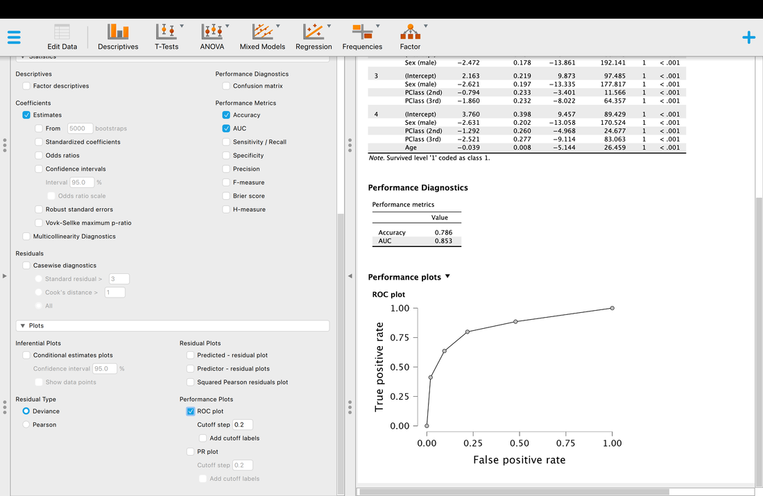
Another thing you may wish to examine is classification accuracy.
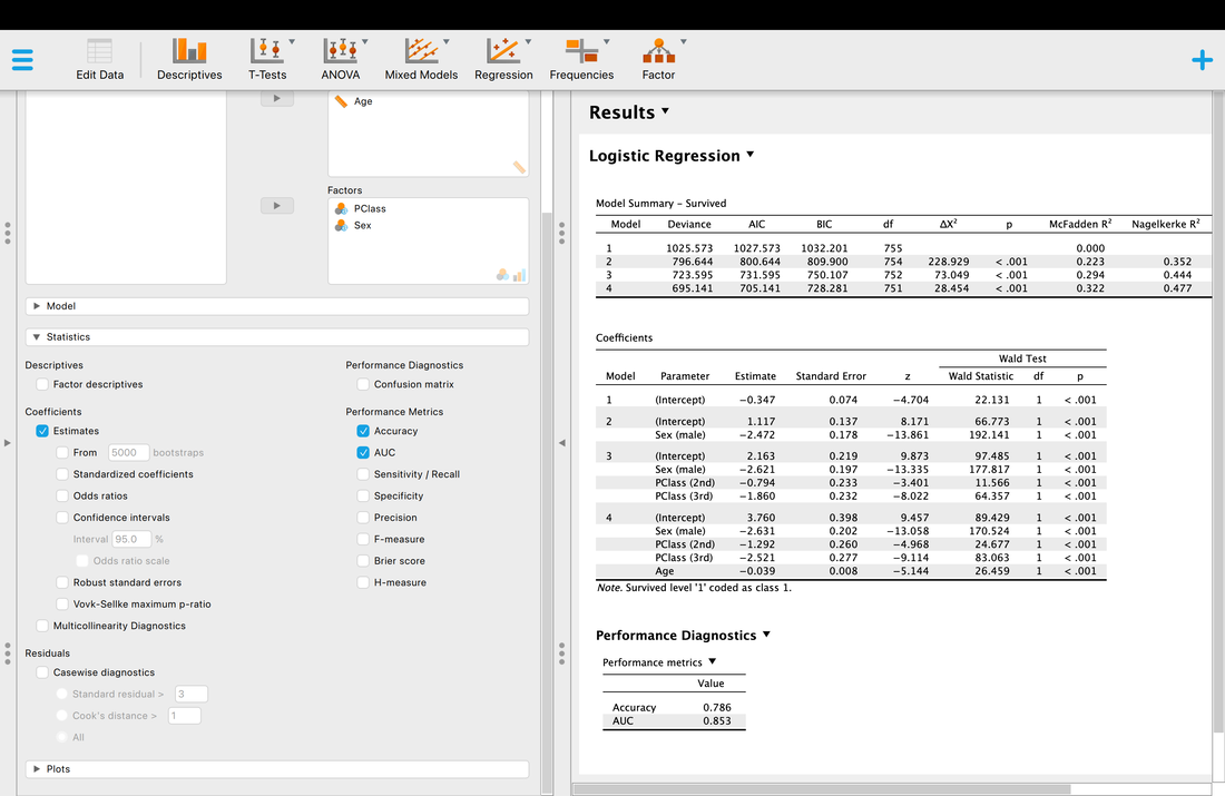
Accuracy is what it is, but what is AUC? AUC is the Area Under the Curve (the ROC curve). Basically, it describes the accuracy of the model. A value of 1 would mean 100% classification accuracy. A value of 0 would mean 0% classification accuracy. The ROC curve is just a way of visualizing the classification accuracy. More on this HERE.
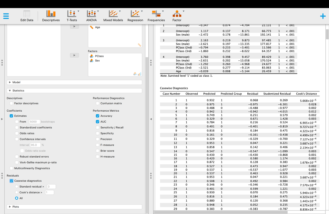
Finally, if you wish you can look at all the individual classifications with information about classification accuracy, whether or not they are outliers, etc.
Assignment
HERE is a data set where 20 EEG variables are being used to predict whether or not someone has MCI (coded no/yes). Run a binary logistic regression, determine which variables are "important", test the assumptions, and examine the classification accuracy.
HERE is a data set where 20 EEG variables are being used to predict whether or not someone has MCI (coded no/yes). Run a binary logistic regression, determine which variables are "important", test the assumptions, and examine the classification accuracy.